Section 7.4: The Distribution of the Sample Proportion
Learning Objectives
1.Describe and interpret the sampling distribution for sample proportions.
2.Compute and interpret probability for a sample proportion.
Chapter 7 is written to summarize continuous random variables and their sampling distributions. So far, we have only discussed quantitative variables: Wait times for trains, lifespan of cell phones, weights of chocolate bars, etc. Our next step is to develop a method to view qualitative variables with the same types of methods. We will do this through random sampling and counting the numbers in the sample that have a qualitative characteristic, then computing the sample proportions with that characteristic. This process creates a new sampling variable that is technically not continuous, but can be approximated using the normal distribution, which is continuous.
Sample Proportions
Definition 1
Assume we wish to measure the proportion or percentage of a sample that has a qualitative characteristic. Let X be the number of observations with the characteristic in a sample of size n.
Then the statistic is the proportion of observations in the sample with the characteristic. The statistic is called the sample proportion, and it is a statistical approximation to the parameter p, the population proportion.
(Note that X is a binomial random variable: X counts the number of successes (an individual in the sample has the characteristic) in n trials (for sample size of size n). See Table 1 for common statistics and parameters they approximate.
Table 1: Common Statistics and Parameters | ||
|---|---|---|
Measurement | Statistic (from a sample) | Parameter (from the population) |
Mean | (x-bar) | (mu) |
Standard Deviation | s | (sigma) |
Proportion of successes in n trials of a binomial experiment. | (p-hat) | p |
Example 1: Computing a Sample Proportion
Pew Research Center conducted a Race in America survey in 2019. One question in the survey asked the respondent to select the best completion to the statement, “In general, the fact that the U.S. population is made up of people of many different races and ethnicities _________ ”
•Has a positive impact on the country’s culture.
•Has a negative impact on the country’s culture.
•Doesn’t make much of a difference.
The survey had 3,314 responses and 2121 selected “Has a positive impact on the country’s culture”. Calculate the sample proportion of responses for “Has a positive impact on the country’s culture”.
Solution:This could have been a question in chapter 5. The sample proportion is simply the probability that a randomly selected person selected “Has a positive impact on the country’s culture”.
So, . From this sample of n = 3314, about 64% of them believe that the ethnic and racial makeup of our country has a positive impact on our culture.
Now, if we took another random sample of a different group of 3314 people, the sample proportion would likely be different. If we took a second sample and found 2185 people who selected “Has a positive impact”, then the sample proportion would have been . Yet a third sample might have had 2115 select “Has a positive impact”, with a resulting sample proportion . Each sample we take will have a different sample proportion. If we create all possible sample proportions and their probability, we have created the distribution of sample proportions.
Table 2 contains 100 simulated samples for surveys of 3314 individuals. Each simulated survey was given to 3314 individuals and reports the number of “Has a positive impact on the country’s culture” responses and the sample proportion. You can open the Table 2 data (opens in a new tab) in STATBELT (download CSV).
Table 2: Simulated Sample Proportion for the Number of "Has a positive impact" responses (n = 3314) | |||||||||||
|---|---|---|---|---|---|---|---|---|---|---|---|
Sample Number | Positive Impact | Sample Proportion | Sample Number | Positive Impact | Sample Proportion | Sample Number | Positive Impact | Sample Proportion | Sample Number | Positive Impact | Sample Proportion |
1 | 2185 | 0.6593 | 26 | 2136 | 0.6445 | 51 | 2101 | 0.6340 | 76 | 2115 | 0.6382 |
2 | 2115 | 0.6382 | 27 | 2100 | 0.6337 | 52 | 2106 | 0.6355 | 77 | 2090 | 0.6307 |
3 | 2085 | 0.6291 | 28 | 2095 | 0.6322 | 53 | 2152 | 0.6494 | 78 | 2113 | 0.6376 |
4 | 2081 | 0.6279 | 29 | 2065 | 0.6231 | 54 | 2119 | 0.6394 | 79 | 2071 | 0.6249 |
5 | 2125 | 0.6412 | 30 | 2119 | 0.6394 | 55 | 2093 | 0.6316 | 80 | 2156 | 0.6506 |
6 | 2136 | 0.6445 | 31 | 2125 | 0.6412 | 56 | 2064 | 0.6228 | 81 | 2134 | 0.6439 |
7 | 2117 | 0.6388 | 32 | 2157 | 0.6509 | 57 | 2067 | 0.6237 | 82 | 2135 | 0.6442 |
8 | 2176 | 0.6566 | 33 | 2124 | 0.6409 | 58 | 2139 | 0.6454 | 83 | 2162 | 0.6524 |
9 | 2125 | 0.6412 | 34 | 2110 | 0.6367 | 59 | 2136 | 0.6445 | 84 | 2134 | 0.6439 |
10 | 2076 | 0.6264 | 35 | 2119 | 0.6394 | 60 | 2110 | 0.6367 | 85 | 2093 | 0.6316 |
11 | 2121 | 0.6400 | 36 | 2084 | 0.6288 | 61 | 2125 | 0.6412 | 86 | 2151 | 0.6491 |
12 | 2153 | 0.6497 | 37 | 2123 | 0.6406 | 62 | 2095 | 0.6322 | 87 | 2159 | 0.6515 |
13 | 2093 | 0.6316 | 38 | 2126 | 0.6415 | 63 | 2121 | 0.6400 | 88 | 2181 | 0.6581 |
14 | 2150 | 0.6488 | 39 | 2119 | 0.6394 | 64 | 2095 | 0.6322 | 89 | 2175 | 0.6563 |
15 | 2153 | 0.6497 | 40 | 2139 | 0.6454 | 65 | 2135 | 0.6442 | 90 | 2132 | 0.6433 |
16 | 2137 | 0.6448 | 41 | 2151 | 0.6491 | 66 | 2125 | 0.6412 | 91 | 2151 | 0.6491 |
17 | 2104 | 0.6349 | 42 | 2130 | 0.6427 | 67 | 2136 | 0.6445 | 92 | 2110 | 0.6367 |
18 | 2091 | 0.6310 | 43 | 2109 | 0.6364 | 68 | 2059 | 0.6213 | 93 | 2074 | 0.6258 |
19 | 2093 | 0.6316 | 44 | 2133 | 0.6436 | 69 | 2133 | 0.6436 | 94 | 2071 | 0.6249 |
20 | 2106 | 0.6355 | 45 | 2079 | 0.6273 | 70 | 2092 | 0.6313 | 95 | 2092 | 0.6313 |
21 | 2086 | 0.6295 | 46 | 2134 | 0.6439 | 71 | 2108 | 0.6361 | 96 | 2114 | 0.6379 |
22 | 2043 | 0.6165 | 47 | 2150 | 0.6488 | 72 | 2136 | 0.6445 | 97 | 2096 | 0.6325 |
23 | 2083 | 0.6285 | 48 | 2068 | 0.6240 | 73 | 2126 | 0.6415 | 98 | 2143 | 0.6467 |
24 | 2127 | 0.6418 | 49 | 2081 | 0.6279 | 74 | 2123 | 0.6406 | 99 | 2134 | 0.6439 |
25 | 2098 | 0.6331 | 50 | 2106 | 0.6355 | 75 | 2118 | 0.6391 | 100 | 2172 | 0.6554 |
Example 2: Describing the Distribution of the Sample Proportion
Use the simulated sample data in Table 2 to make a histogram of the sample proportions for the 100 samples. Find the mean and standard deviation for the sample proportions. Describe the distribution of sample proportions. You can open the Table 2 data (opens in a new tab) in STATBELT (download CSV).

Photo by Husna Miskandar (opens in a new tab) on Unsplash (opens in a new tab)
Solution:Open STATBELT Utility. Open the data using the link, copy the values in the “Positive Impact” and “Sample Proportion” columns (not the column names), and paste them into the first two columns of the spreadsheet. Type “Positive Impact” and “Sample Proportion” in the column headings. You can ignore the “sample number” column.
To make the histogram, select Graphs → Histogram, and choose “Sample Proportion” for the column. You can type the start and bin width or let STATBELT choose them for you. Click “Open graph in a new window.” The histogram is shown in figure 7.29.
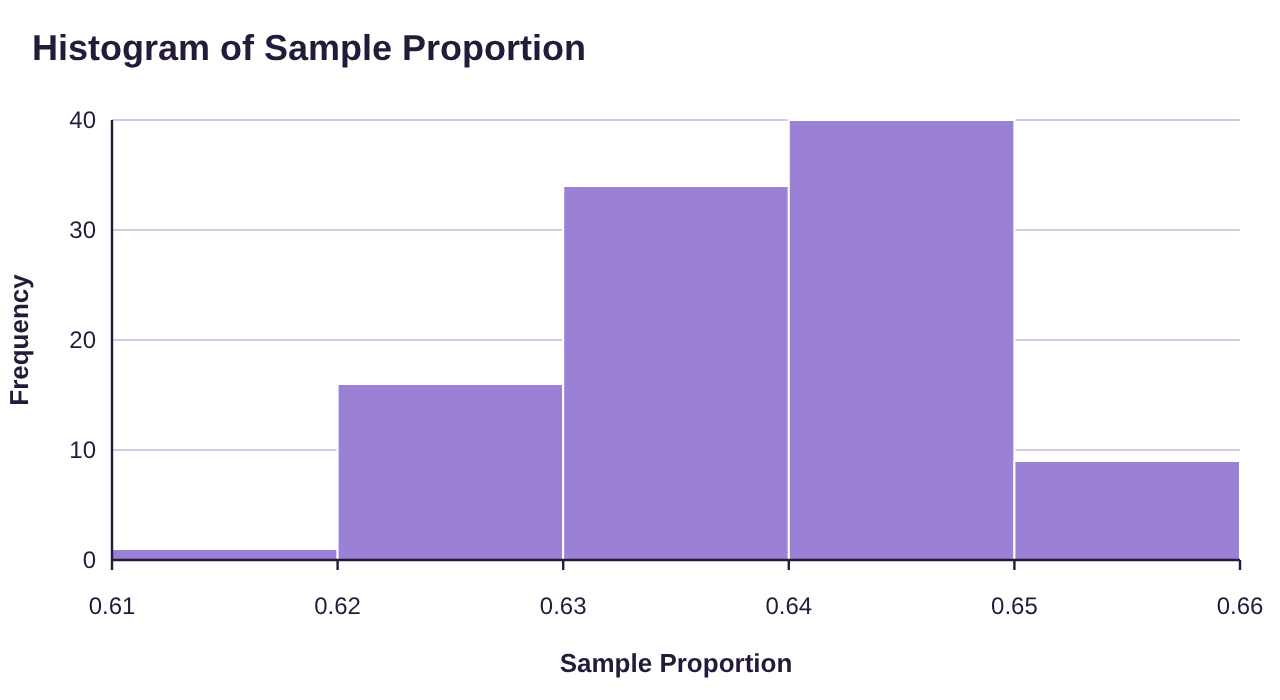
Figure 7.29: Histogram for simulated sample proportions.
You may not be surprised to see that the distribution of sample proportions looks bell-shaped. The distribution will be normal under the right conditions, which we will present shortly.
To get the mean and standard deviation, you can select Descriptive Statistics → Basic Statistics, check “Sample Proportion” under “Columns to include,” and click “Show results in a new window,” as we did in chapter 3. The mean is given as 0.6388, and the standard deviation is given as 0.0089.

Another option is to mark the mean on the histogram. When you choose Graphs → Histogram and choose “Sample Proportion”, check “Show mean (x̄) in green.” The histogram then shows a green triangle at the mean, labeled with its value. STATBELT does not draw a normal curve over a histogram, so we judge the bell shape by eye. See figure 7.30.
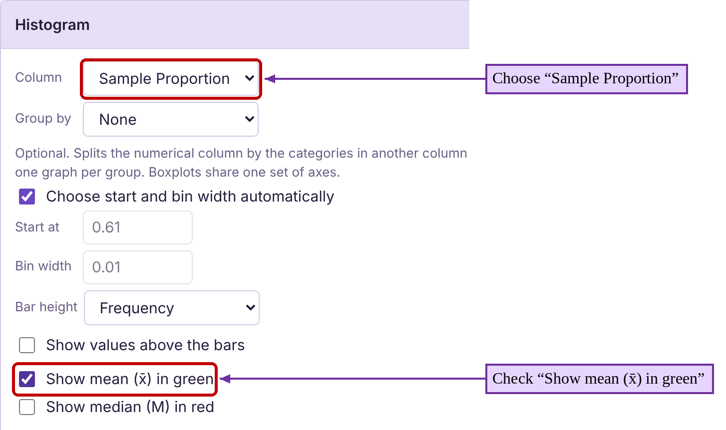

Photo by Joel Muniz (opens in a new tab) on Unsplash (opens in a new tab)
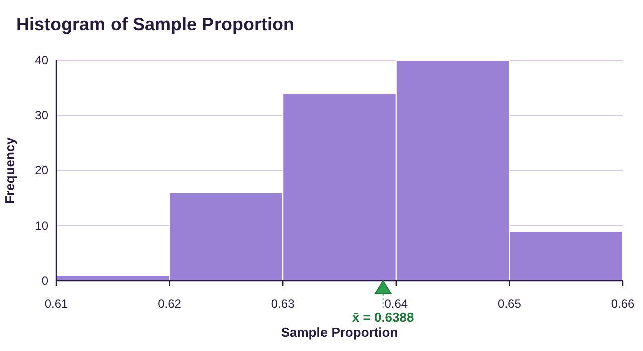
Figure 7.30: Histogram for simulated sample proportions with the mean marked.
Once again, we see that the mean is 0.6388, and Basic Statistics gave the standard deviation as 0.0089.
So, it appears that the distribution of sample proportions has the following description:
•Center- The mean is approximately .
•Variation- The standard deviation is approximately 0.0089.
•Shape- The distribution appears to be normally distributed.
What we have seen so far is that if we consider the distribution of sample proportions, it appears to follow a bell shaped distribution. But is that always the case? Sadly, no.
Example 3: Computing Sample Proportions for the Number of Twos in 10 Dice Rolls
Recall that in section 7.3, example 2, a nutty professor rolled 10 dice 100 times. He recorded the numbers of each face that appeared. If we let X = the number of twos out of the 10 dice in each sample, then X is a binomial variable.
The first sample result was {2, 2, 3, 3, 3, 3, 4, 4, 5, 5}.
The second sample result was {1, 1, 1, 2, 3, 5, 6, 6, 6, 6}.
The third sample result was {1, 2, 2, 3, 4, 4, 4, 5, 5, 6}.
Find the sample proportion for the number of twos in each of the first three samples and compare them.
Use the data in Table 3 to create a histogram for the sample proportions of the number of twos out of 10 rolls for all 100 samples. Verify that it is not a normal distribution.
Solution:In the first sample, there were X = 2 twos, so the sample proportion is .
The second sample had only X = 1 two, so the sample proportion for that sample is
The third sample had X = 2 twos, so the sample proportion for that sample is .
The theoretical probability of rolling a two is . The sample proportions we have are 0.2, 0.1, and 0.2. These sample proportions cannot be equal to 1/6 because the sample size is 10, so all sample proportions will be tenths. But the mean of the first three sample proportions is
So, it appears that the mean of the sample proportions is close to the probability of rolling a two. This makes sense. Rolling dice and counting the number of twos is a binomial experiment with expected value twos per roll of 10 dice. Some samples will have more twos, and some will have fewer. But they will average out to about 1.667 twos per sample of 10, giving a proportion of , which is also the probability of rolling a two in one roll. (The mean of the distribution of sample proportions equals the probability of success in the binomial experiment!)
Table 3 contains the sample proportions for all 100 samples of size n = 10. You can open the Table 3 data (opens in a new tab) in STATBELT (download CSV). If you make a histogram of the sample proportions, we can see that it is skewed to the right. See figure 7.31.
Table 3: Sample Proportion for the Number of Twos obtained in 100 Samples of 10 Six-sided Dice Rolls | |||||||||||
|---|---|---|---|---|---|---|---|---|---|---|---|
Sample Number | Number of Twos | Sample Proportion | Sample Number | Number of Twos | Sample Proportion | Sample Number | Number of Twos | Sample Proportion | Sample Number | Number of Twos | Sample Proportion |
1 | 2 | 0.2 | 26 | 0 | 0 | 51 | 1 | 0.1 | 76 | 3 | 0.3 |
2 | 1 | 0.1 | 27 | 1 | 0.1 | 52 | 1 | 0.1 | 77 | 0 | 0 |
3 | 2 | 0.2 | 28 | 1 | 0.1 | 53 | 1 | 0.1 | 78 | 2 | 0.2 |
4 | 1 | 0.1 | 29 | 1 | 0.1 | 54 | 1 | 0.1 | 79 | 2 | 0.2 |
5 | 2 | 0.2 | 30 | 4 | 0.4 | 55 | 2 | 0.2 | 80 | 3 | 0.3 |
6 | 2 | 0.2 | 31 | 0 | 0 | 56 | 2 | 0.2 | 81 | 2 | 0.2 |
7 | 1 | 0.1 | 32 | 1 | 0.1 | 57 | 0 | 0 | 82 | 0 | 0 |
8 | 2 | 0.2 | 33 | 0 | 0 | 58 | 0 | 0 | 83 | 2 | 0.2 |
9 | 3 | 0.3 | 34 | 0 | 0 | 59 | 2 | 0.2 | 84 | 2 | 0.2 |
10 | 2 | 0.2 | 35 | 5 | 0.5 | 60 | 4 | 0.4 | 85 | 1 | 0.1 |
11 | 1 | 0.1 | 36 | 1 | 0.1 | 61 | 1 | 0.1 | 86 | 4 | 0.4 |
12 | 3 | 0.3 | 37 | 2 | 0.2 | 62 | 1 | 0.1 | 87 | 0 | 0 |
13 | 3 | 0.3 | 38 | 1 | 0.1 | 63 | 3 | 0.3 | 88 | 3 | 0.3 |
14 | 1 | 0.1 | 39 | 2 | 0.2 | 64 | 3 | 0.3 | 89 | 0 | 0 |
15 | 2 | 0.2 | 40 | 0 | 0 | 65 | 1 | 0.1 | 90 | 3 | 0.3 |
16 | 1 | 0.1 | 41 | 1 | 0.1 | 66 | 0 | 0 | 91 | 1 | 0.1 |
17 | 1 | 0.1 | 42 | 2 | 0.2 | 67 | 4 | 0.4 | 92 | 3 | 0.3 |
18 | 0 | 0 | 43 | 1 | 0.1 | 68 | 1 | 0.1 | 93 | 0 | 0 |
19 | 2 | 0.2 | 44 | 2 | 0.2 | 69 | 1 | 0.1 | 94 | 3 | 0.3 |
20 | 1 | 0.1 | 45 | 0 | 0 | 70 | 5 | 0.5 | 95 | 0 | 0 |
21 | 1 | 0.1 | 46 | 3 | 0.3 | 71 | 2 | 0.2 | 96 | 1 | 0.1 |
22 | 3 | 0.3 | 47 | 4 | 0.4 | 72 | 3 | 0.3 | 97 | 1 | 0.1 |
23 | 3 | 0.3 | 48 | 2 | 0.2 | 73 | 1 | 0.1 | 98 | 0 | 0 |
24 | 3 | 0.3 | 49 | 2 | 0.2 | 74 | 3 | 0.3 | 99 | 2 | 0.2 |
25 | 1 | 0.1 | 50 | 3 | 0.3 | 75 | 1 | 0.1 | 100 | 4 | 0.4 |
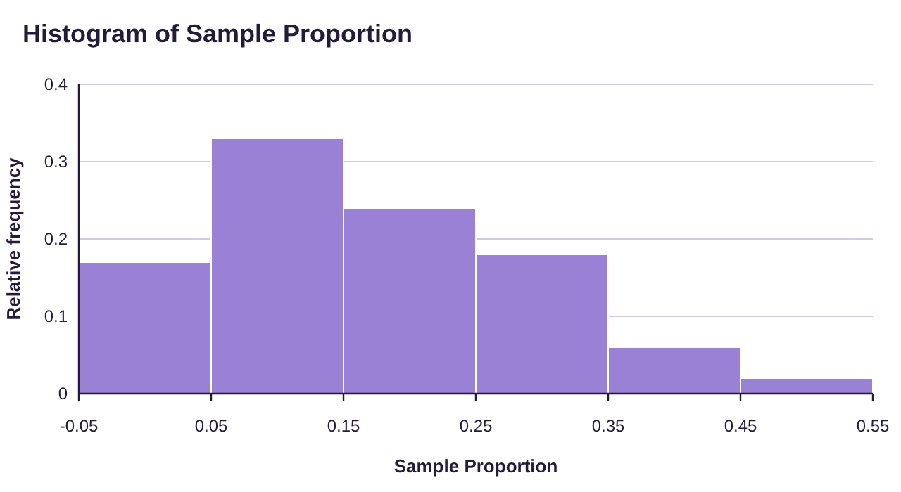
Figure 7.31: Histogram for sample proportions for the number of Twos in 10 rolled dice.
The histogram looks like it is a little bell-shaped, but not close enough for us to call it a normal distribution. This shows that the distribution of sample proportions is not normal in this case.
So, why is the distribution of sample proportions normal in example 2, but not in example 3? The answer has to do with the binomial random variable X. We created by dividing the binomial variable X by n. Dividing by n merely changes the vertical scale on the distribution but does not affect the shape. So, if X is approximately normally distributed, then is too. We saw in section 6.3 that a binomial random variable X will have a bell-shaped distribution if .
In example 1, we had n = 3314 and p = 0.64 (approximated), so
This confirms that X is approximately normally distributed, and so is as well.
In example 3, we had n = 10 and p = 1/6, so
This shows that X is not bell-shaped, so neither X nor are approximately normally distributed.
Central Limit Theorem (CLT) for Proportions
Assume that random samples of size n are taken from a population with a population proportion p (this is a parameter). The sampling distribution for the sample statistic has the following characteristics:
1.Center- The mean is
2.Variation- The standard deviation is
3.Shape- The distribution will be approximately normal if .
The larger n is, the closer to normal the distribution for gets.
* Note that additionally, to ensure that X is a binomial random variable, we need to know that the trials are independent. That means that the sample size must be less than 5% of the population size.

Important Point!
The distribution of sample proportions can be used to find probability relating to sample proportions. However, remember that this is a normal approximation to it, so the probability you find using this distribution is an approximation. If you need the exact probability for a binomial random variable, using the binomial calculator is a better choice. In that case, you might wonder, why do we study this approximation? There are two reasons.
•Before numerical methods like calculators and STATBELT existed, using z-scores, tables of area, and approximations to the normal curve was much easier than computing binomial probability for “”, “”, and “between” probabilities by hand. In those cases, using the normal approximation could save hours of tedious work! Although the historic reason is nice to know, the second reason is more important to us now.
•The distribution of the sample proportion is used for inference. When we work with inference, we generally work with population proportions that we treat as continuous and normally distributed, rather than discrete variables. We will use the distribution of sample proportions to find margins of error, reject suspicious claims, estimate population proportions that are unknown, etc. These topics, and more, will be covered in Unit 3, chapters 8, 9, 10 and 11.
Example 4: Computing the Mean and Standard Deviation for the Sample Proportion of the Number of Twos in 10 Dice Rolls
Revisiting example 3, recall that the professor rolled 10 dice 100 times and recorded the number of twos in each roll of 10 dice. We let X = the number of twos out of the 10 dice in each sample, and is the proportion of twos in each sample. Find the mean and standard deviation for the distribution of sample proportions. Compare them to the mean and standard deviation from the 100 sample proportions in Table 3.
Solution:We will leave it to the reader to check that the variable X is binomial, with n = 10 and p = 1/6.
•According to the central limit theorem, the mean of the distribution is . (When we found the mean of the first three sample proportions in example 3, the result was already exactly 1/6.) The mean of the 100 sample proportions in Table 3 is 0.169, which is very close to . See figure 7.32. The mean of the sample proportions appears to be equal to p = 1/6 based on the experiment.
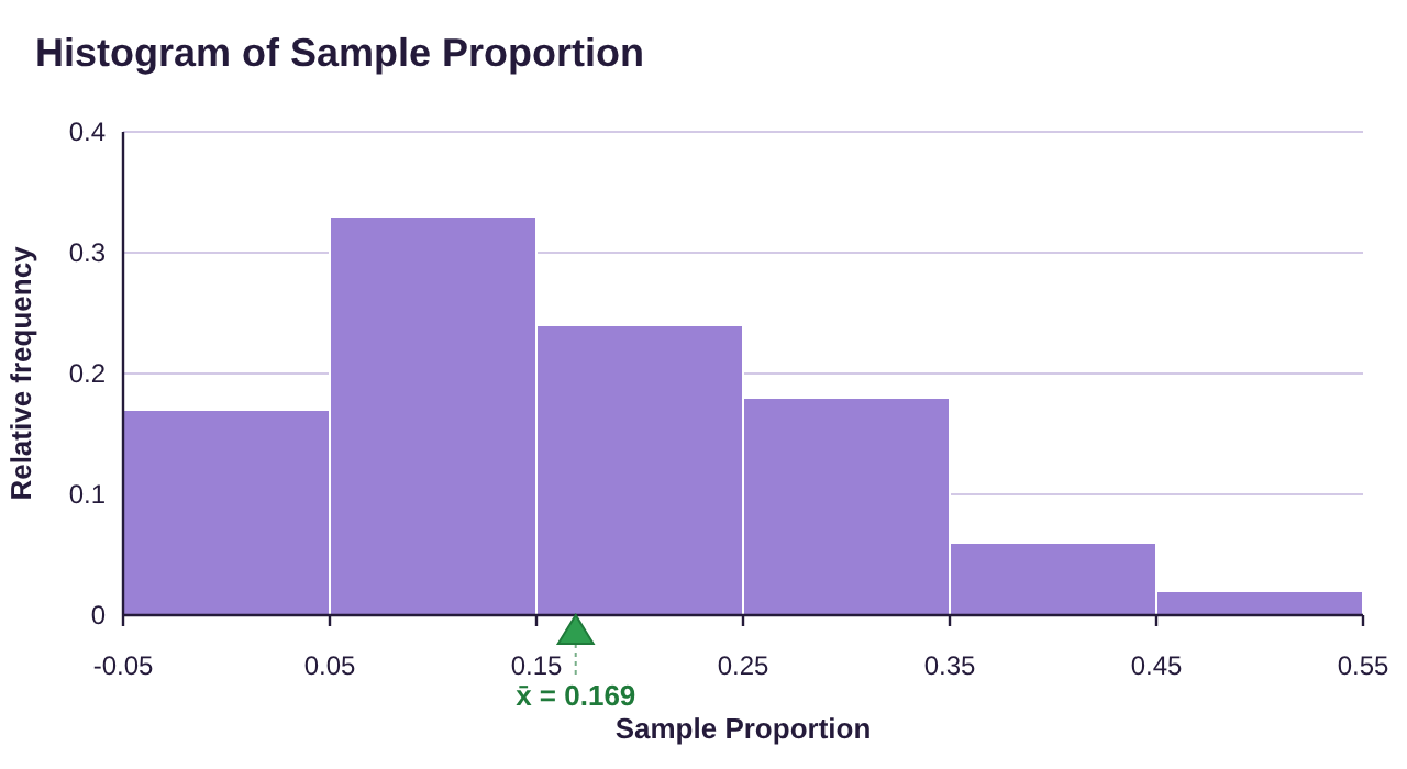
Figure 7.32: Histogram for sample proportions for the number of Twos in 10 rolled dice, with the mean marked.
•The standard deviation for the distribution of sample proportions is . If we substitute n = 10 and p = 1/6, we get
The theoretical standard deviation for the distribution of sample proportions is approximately 0.1179. The standard deviation from the 100 samples was 0.1237. These are close as they both round off to 0.12 at two decimal places. This suggests that the formula for the standard deviation given in the central limit theorem for proportions is reasonable.
We have already noted that the distribution in this case is not normal, so we have described the center using the mean, the variation using the standard deviation, and the shape as not normal.
Example 5: Describing the distribution of Sample Proportions
According to the U.S. Public Interest Research Group’s Education Fund report, 65% of college students in the U.S. have skipped purchasing textbooks for their classes due to cost, despite concerns about their grades. Assume that samples of size 160 are randomly selected from the population of college students in the U.S. Let be the proportion that have skipped purchasing textbooks. Describe the sampling distribution of sample proportions.

Photo by Daria Nepriakhina 🇺🇦 (opens in a new tab) on Unsplash (opens in a new tab)
Solution:To describe the sampling distribution for sample proportions , we need to know the population proportion p and the sample size n. In this example, it is reported that 65% of college students skip purchasing textbooks due to the cost, so we will use p = 0.65. Random samples of size n = 160 are taken.
•The mean is .
•The standard deviation must be calculated.
•To determine the shape, we check if .
Since , the distribution of sampling proportions will have an approximately normal distribution.
 Tip!
Rounding and decimal places: Since sample proportions are computed as a probability (the number with a characteristic divided by the total), and we have been rounding probability to 4 decimal places throughout the book, we also round sample proportions to 4 decimal places. When we compute the standard deviation, we usually want it rounded to one or two places more than the mean. But here, the mean is a proportion rounded to 4 places, so we will round the standard deviation to 5 or 6 decimal places. If you round off with fewer places, it may cause your answers from probability calculators to be slightly incorrect. As a rule, round off only at the end of all calculations!
Example 6: Describing the distribution of Sample Proportions
According to the Institute for Health Metrics and Evaluation (IHME), approximately 82% of the U.S. population has been infected with COVID-19 at least once as of July 2022. Assume that samples of size n = 200 are randomly selected from the U.S. population.
a)Describe the distribution of sample proportions for those who have been infected with COVID-19.
b)Use the sampling distribution to estimate the probability that a sample would have less than 75% with COVID-19 infections.
c)Use the sampling distribution for the sample proportion to estimate the probability that a sample of 200 would have 175 or more COVID-19 infections.
Solution:a)To describe the sampling distribution for sample proportions , we need to know the population proportion p and the sample size n. In this example, it is reported that 82% of the population has been infected with COVID-19 at least once, so p = 0.82. Random samples of size n = 200 are taken.
◦The mean is .
◦The standard deviation is calculated as follows.
◦To determine the shape, we check if .
Since , the distribution of sampling proportions will have an approximately normal distribution.
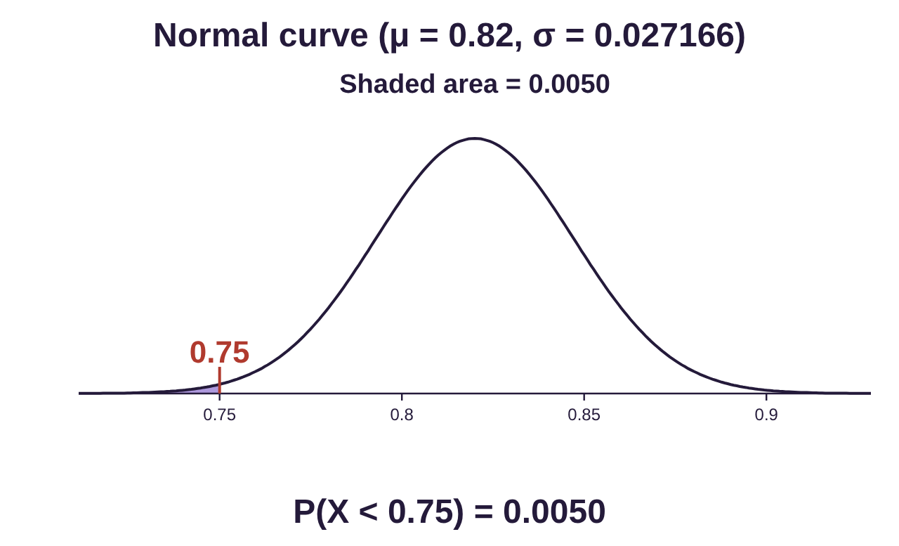
b)Since we know the distribution of sample proportions has a normal distribution with mean and standard deviation , we can use a normal calculator. Open STATBELT Utility and select Calculators → Normal Calculator. Type in the mean as and standard deviation as . Symbolically, the probability that a sample proportion is less than 75% is
. Choose “P(X < a)” and type 0.75 for the value a. The result is , or 0.0050 rounded to 4 decimal places.
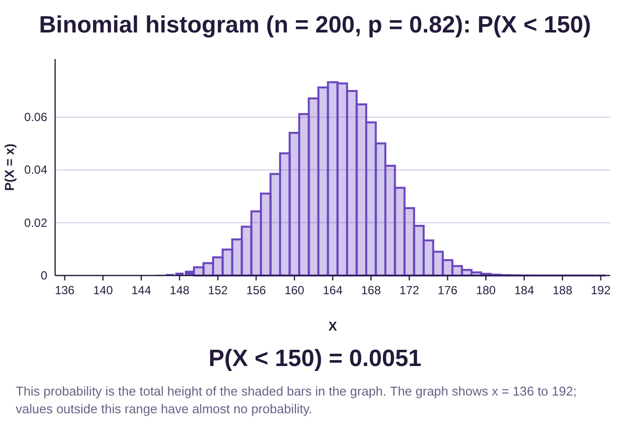
Note on part b): If we treat X as binomial, then we can answer part (b) using the binomial calculator and get the exact answer rather than the approximation. Since 75% of 200 is 150, having a sample proportion less than 75% means the same as having X < 150. The exact answer using n = 200 and p = 0.82 is , which is very close to the answer we found before. Don’t forget that the binomial calculator can give the exact probability where the normal approximation to the distribution of sample proportions gives us a close approximation!
Tip!When a sample or population proportion is given as a percentage, you must convert it to decimal form! In this example, we are given 82% had COVID-19, but we use the decimal equivalent 82% = 0.82 when we report the mean and calculate the standard deviation. When we are asked to find the probability that a sample proportion is less than 75%, we use the decimal equivalent of 75% = 0.75. Percent form can be used to summarize a population, or to describe a conclusion, but should not be used for calculations along the way! Should you ever get a very odd answer or error message when working through computations, check that you converted your percentages into decimal form!
c)In part c) we are asked to use the distribution of sample proportions to estimate the probability that a sample would have 175 or more COVID-19 infections. We start with and convert this statement to a statement about the sample proportion. To do this, we divide each side of the inequality by the sample size n = 200.
divide both sides by 200
since and
So . Using the normal calculator with mean 0.82 and standard deviation 0.027166 we choose “P(X > a)” and type 0.875 for the value a. The result is rounded to 4 decimal places.
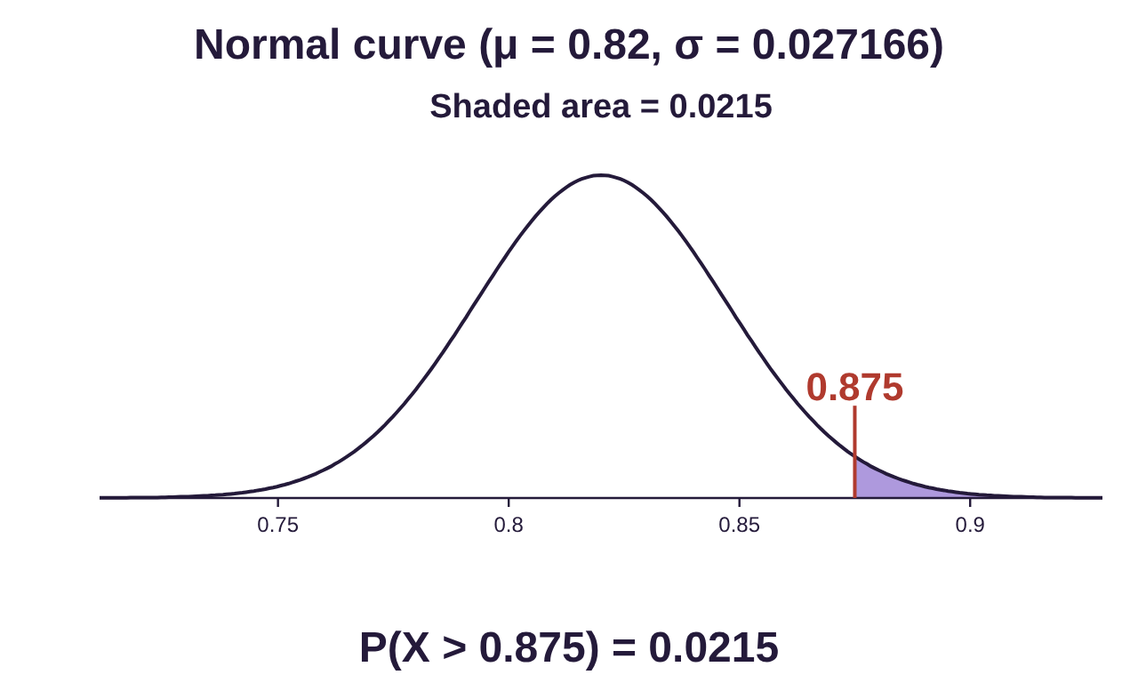
Note that if we had used the binomial calculator instead, we could have found directly, and it would have been the exact answer rather than the approximation given by the normal curve. The exact answer is .
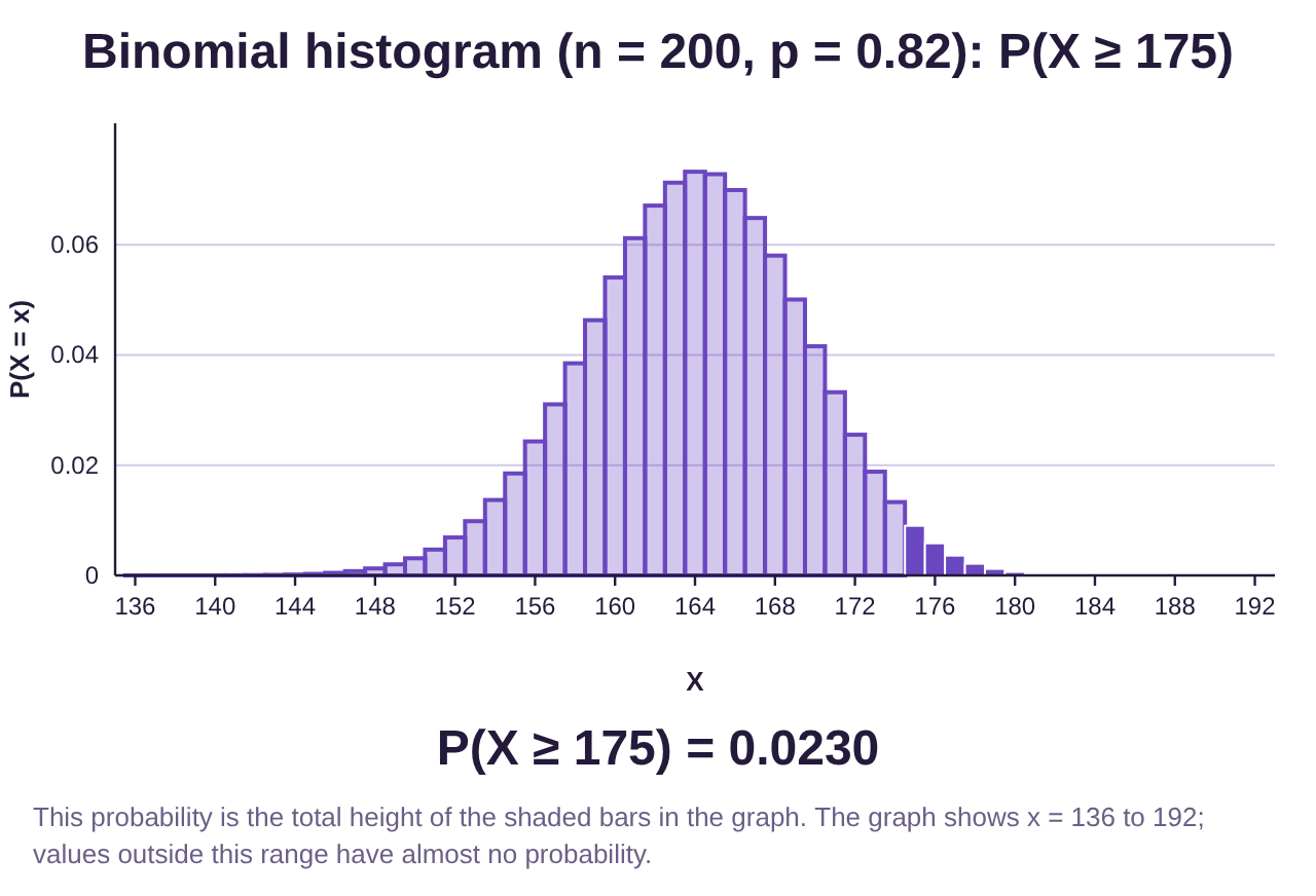
Once again, using the distribution of the sample proportions gave us a very close approximation to the answer we could find directly using the binomial calculator, 0.0215 compared to 0.0230.

Photo by Tony Tran (opens in a new tab) on Unsplash (opens in a new tab)