Section 5.1: Basic Probability

Probability forms the basis of inferential statistics. But what is probability? Most of us have some sense of it from flipping a coin or from weather reports giving the chance of rain. We intuitively know that a coin flip has a 50% chance of coming up tails. We understand that a 90% chance of rain means that rain is likely, but how will that help us to make inferences from data? First, we need some definitions.

There are three approaches we can take to establish the likelihood of an event. Here is an overview.

1. Theoretical (or classical) probability:

If the outcomes of an event are equally likely, we can make a list of all the possible outcomes. This is called a sample space, and we can calculate the proportion of times the desired event will occur theoretically. But this approach can only be used when you can create a sample space of equally likely outcomes! Sadly, this is not the case when we study social issues. But it is useful for studying games like poker, dice, or roulette.

2. Empirical (or experimental) probability:

Empirical probability is another name for the relative frequency we worked with in chapter 2. We can repeat an experiment many times and calculate the proportion of times the event occurs or find the relative frequency from collected data. We would use this to estimate the chances of being involved in car crash, catching Covid-19, or graduating high school. It would not be possible to establish these probabilities theoretically because it is impossible to write out a list of equally likely outcomes.

3. Subjective probability:

Subjective probability is making an informed guess in situations when you cannot repeat an experiment, and you cannot create a sample space of equally likely outcomes. For example, the probability that it will rain cannot be computed either of the first two ways, so we create computer models that effectively help us make very good guesses as to the chance of rain. But it is still a guess.

Next, we will take a closer look at each type of probability.

Theoretical Probability

To use theoretical probability, we need to create a list of all possible outcomes of the activity, or experiment. Additionally, each outcome must have the same chance of occurring, like flipping a coin, rolling dice, or randomly selecting a card from a deck. The probability that the event will happen is then calculated as the number of ways the event can occur, divided by the total number of possible outcomes.

Solution:When you roll a fair six-sided die, all the outcomes are equally likely. That means each face numbered one through six has an equal chance of showing up. So, the sample space is a list of all the equally likely outcomes, in this case {1, 2, 3, 4, 5, 6}. A diagram of the sample space is in figure 5.2.

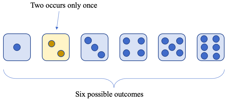
Figure 5.2: Illustration of the sample space for rolling a single six-sided die.

The probability of rolling a two is found by observing the number of times “two” occurs in the sample space, which is only one time. There are a total of 6 possible outcomes.

So, the probability of rolling a two is $P\left(\text{roll }a2\right)=\frac{1}{6}\approx 0.1667$.

Solution:Again, since dice have equally likely outcomes, we can create a sample space and find the answer using theoretical probability. For clarity, let’s assume that one die is blue and the other is red. Each possible outcome of rolling the two dice is the number showing on the blue die, and the number showing on the red die. Figure 5.3 shows all 36 possible outcomes of rolling two dice.

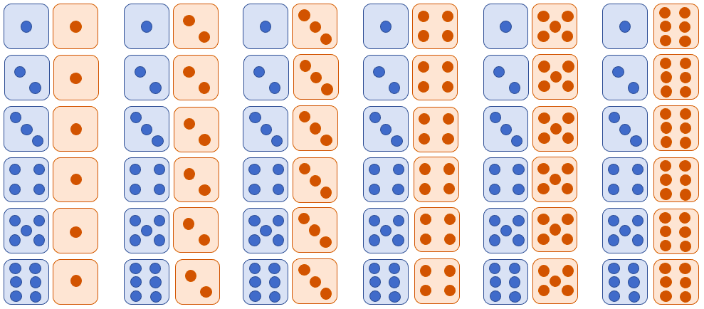
Figure 5.3: Illustration of the sample space for rolling two six-sided dice.

It is important to note that rolling a six on the blue die and a two on the red die is not the same as rolling a two on the blue die and a six on the red die. Since the numbers on the dice are switched, they are different outcomes, even though they are both a six and a two.

a)To calculate the probability of rolling double sixes, note that there is only one way to do that listed in the sample space, highlighted in figure 5.4.

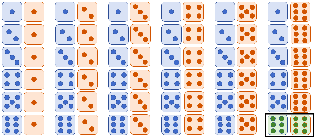
Figure 5.4: There is only one outcome that is double sixes.

So, the probability of rolling double sixes is

$$\begin{array}{cc}P\left(\text{double sixes}\right)& =\frac{1}{36}\approx 0.0278.\end{array}$$

b)To calculate the probability that the sum is 8, we find the number of ways the sum of 8 occurs in the sample space and divide it by the total number of outcomes. There are 5 ways to get a sum equal to 8, highlighted in figure 5.5.

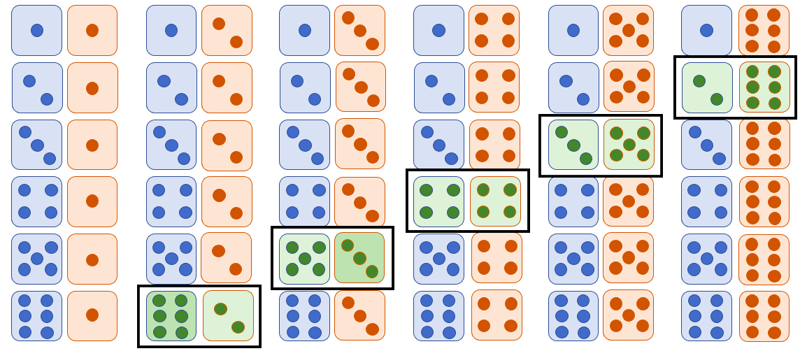
Figure 5.5: The ways rolling two six-sided dice gives a sum equal to 8.

Thus, the probability that the sum is 8 is

$$P\left(\text{sum equals }8\right)=\frac{5}{36}\approx 0.1389\text{.}$$

We can express the probability as a percent and say that rolling two six-sided dice will result in a sum equal to 8 about 13.89% of the time.

c)There are no sums of two dice that equal to 1. All the sums are at least 2. So, rolling a sum that is equal to 1 is impossible and will never happen. The probability of getting a sum equal to 1 is then calculated as zero out of thirty-six, or

$$\begin{array}{cc}& P(\text{sum equals }1)=\frac{0}{36}=0\mathrm{.}\end{array}$$

We interpret this probability as saying the probability is zero, or there is a zero-percent chance it will happen.

d)Since every sum is at least two, getting a sum that is at least two will happen every time. That is, it will happen 36 out of 36 times, so the probability is

$$\begin{array}{cc}& P(\text{sum equals at least }2)=\frac{36}{36}=1\mathrm{.}\end{array}$$

Here, saying that the probability equals 1 is equivalent to saying that there is a 100% chance it will happen.

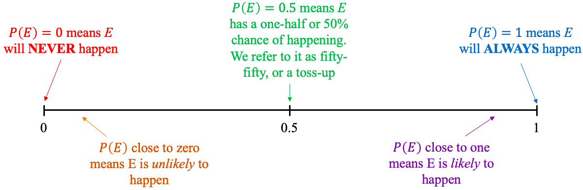
Figure 5.6: The range of probability.

Solution:a)Since each outcome of each coin toss is equally likely, we can use a sample space to answer the question. The easiest way to organize the possible sequences is to use a tree diagram.

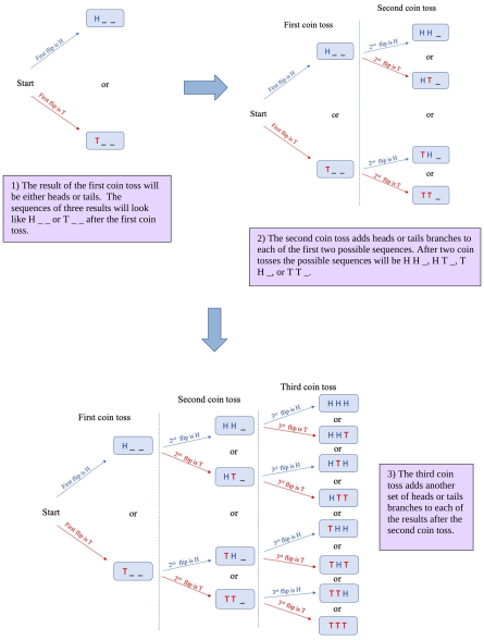
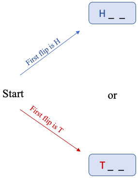
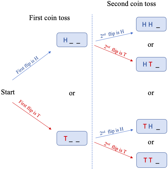
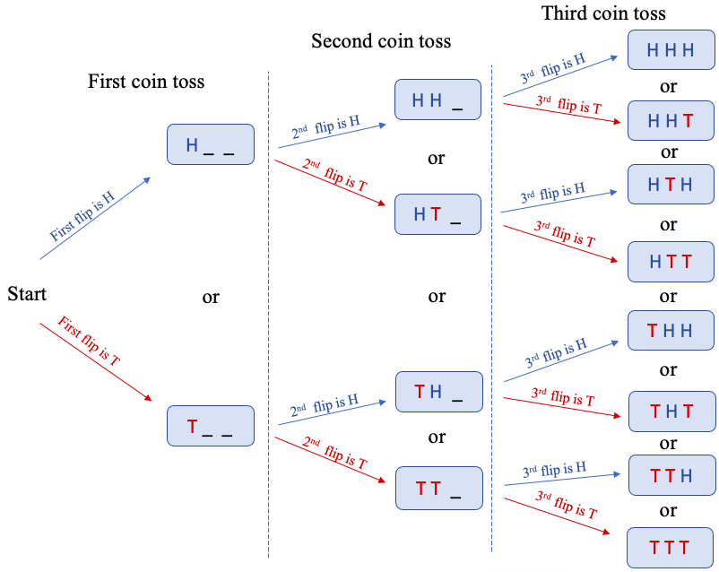
Figure 5.7: Tree diagram for sequence of three coin-flips.

See figure 5.7 for the completed “tree diagram” after three coin-tosses. Tree diagrams are helpful when you need to keep track of sequences of outcomes.

From the tree diagram, we can see that there will be 8 different sequences of three coin flips that are possible. The sample space is S = {HHH, HHT, HTH, HTT, THH, THT, TTH, TTT}.

b)Exactly twice means that there will be two tails and one head in the sequence. Looking at the sample space, we can see that there are three outcomes with exactly two tails, HTT, THT, and TTH.

{HHH, HHT, HTH, HTT, THH, THT, TTH, TTT}

So, the probability of getting exactly two tails is $P\left(\text{exactly two tails}\right)=3/8=0.375$

c)Getting tails at least once means that there is at minimum one tail in the sequence. The only outcome without any tails is the first one, HHH. That means that 7 out of the 8 outcomes have at least one tail.

{HHH, HHT, HTH, HTT, THH, THT, TTH, TTT}

So, the probability is $P\left(\text{at least one tail}\right)=\frac{7}{8}=0.875$

Empirical Probability

Unfortunately, it is not always possible to describe a sample space because there are many occurrences that do not have equally likely outcomes. For example, the probability that a person of color is a homeowner cannot be calculated by creating a sample space because owning a home and not owning a home are not equally likely. If we want to find the probability of this, we must use data to find the relative frequency that a person of color is a homeowner. The new, fancier name for using relative frequency, is called using empirical probability.

Solution:Having no tattoo, one tattoo, or more tattoos are not equally likely events, so we can’t use the theoretical approach. Our only choice is to use the empirical approach to estimate the probability of having no tattoo using the data. From the frequency table we can see that the number of people surveyed with no tattoo is 59. The empirical probability of having no tattoo will be this number divided by the total number of people surveyed.

The total is not given, so we will add the frequencies from the table to find it. The total is 59 + 13 + 35 + 5 = 112. So, the empirical probability is calculated as

$$\begin{array}{cc}P\left(\text{no tattoo}\right)& =\frac{59\text{ with no tattoo}}{112\text{ total}}\approx 0.5267857.\end{array}$$

Usually, we round probability to three or four decimal places. Here, we would write the probability that a randomly selected student has no tattoo is approximately 0.527. We could also express it in a percent form as a 52.7% chance that a student has no tattoo.

Tip!

When we compute empirical probability, we are using data to make the estimate. So, we need to make sure that the data was collected without bias, and we need to collect enough data to deem the results accurate and reliable. For example, if you ask three friends if they have a tattoo, you have a very small sample! Small samples may not be diverse enough to reflect the population. If you collected data from 2,500 people, you can be more confident in the probability you calculate. This is known as the law of large numbers.

To illustrate the Law of Large Numbers, we simulated flipping a coin one-thousand times and graphed the results with STATBELT Utility- the Statistical Basics Exploratory Learning Tool (opens in a new tab). See figure 5.8.

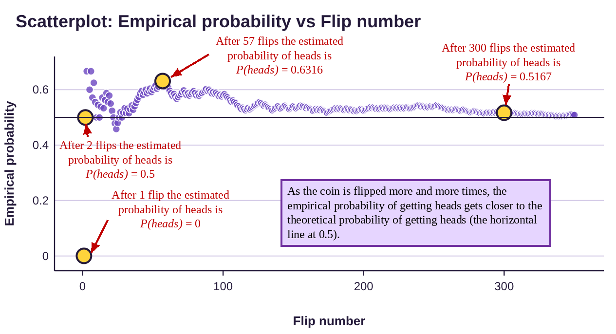
Figure 5.8: Coin flip simulation.

We know that theoretically, the probability of getting Heads is 1/2 = 0.5. We updated the empirical probability after each coin flip and plotted the probabilities in the chart (only up to 350 flips). At first, with fewer coin flips, the probability jumped around. It got as high as 0.6316 after 57 coin-flips, then dropped back down toward 0.5. As you can see, as the number of flips increased, the empirical probability got closer to 0.5.

You can also see the gradual trend toward the theoretical probability by looking at Table 2. After 1 flip, the empirical probability is 0. After 2 flips, it is 0.5. The table includes up to 1000 flips when the empirical probability was calculated to be 0.506.

So, if you can’t find probability theoretically, you can estimate it by collecting data. But you may need a lot of data!

Solution:The two outcomes, whether someone has or has not been unfairly stopped by police are not equally likely. For that reason, we can’t compute this probability theoretically. Instead, we use the data to estimate the probability using the empirical method. Fortunately, it appears there is a large amount of data, so the estimate should be reasonable.

The number of Black Americans who responded “yes” is 668. It is tempting to divide 668 by 802, but 802 was the number who responded “no,” not the total. The total number of Black Americans in the survey was the number who replied “yes” plus the number who replied “no” (there were 48 nonresponses, but we will ignore them for this question). That gives us a total of 668 + 802 = 1,470.

So, the probability that a Black American feels they have been unfairly stopped by police is approximately $\frac{668}{1470}\approx 0.4544$.

In the last example, the probability that a Black American felt they had been unfairly stopped by police was 0.4544. The two interpretations are:

1)There is a 45.44% chance that one randomly selected Black American feels they have been unfairly stopped by police.

2)About 45.44% of all Black Americans feel they have been unfairly stopped by police.

Solution:1)The probability that a given U.S. household subscribes to a cable TV service is 0.44. You can also say there is a 44% chance that one randomly selected U.S. household will be a cable subscriber.

2)Overall, about 44% of U.S. households subscribe to a cable TV service.

Subjective Probability

In situations when we can’t create a sample space, and we can’t run an experiment or collect data, our only option is to make an informed guess as to the likelihood of an event. Of course, any guess we make will be subjective, and hence we call this approach finding a subjective probability. For example, you can’t calculate the probability of a sports team winning a specific game using either the classical or empirical approach. Winning and not winning are not equally likely, so you can’t find it theoretically. Neither can you collect data on how often the team wins the game by playing that specific game over and over to see how often they win it (each repeat would be a new game, played with different factors such as the condition of the players on each team, not the “same game”). The only option is to use subjective assessment of their chances. Even if you use computer simulations, the result is still based on the information the simulations use, which makes it subjective. Sadly, there is no formula for finding subjective probability.

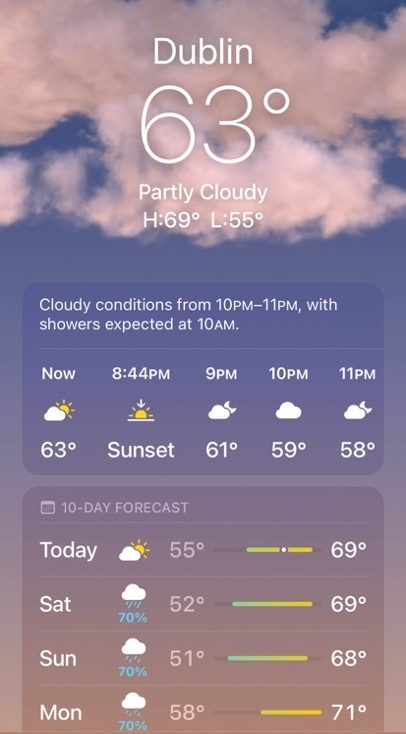
Figure 5.9: The Weather in Dublin, Ireland.

Solution:According to the weather app on my phone, there is a 70% chance that it will rain on Saturday. Once again, this is subjective because it is not based on data collected by repeating Saturday over and over to see how often it rained, nor is it from a sample space. It is subjective! Another weather service might think there is a 60% chance of rain at the same time and at the same location. There is no way to know for certain until Saturday arrives. (But it is Ireland, so you should just assume it is going to rain.)

Properties of Probability

Now that we have looked at the three approaches to calculating probability, we will turn our attention to some of the properties of probability.

Solution:a)We must use empirical probability to estimate this probability. The number of eligible Hispanic voters is 29,210,000. The total number of eligible voters is 233,674,000. So, the probability that an eligible voter is Hispanic is

$$\begin{array}{cc}& P\left(\text{Hispanic}\right)=\frac{\mathrm{29,210,000}}{\mathrm{233,674,000}}\approx 0.1250\mathrm{.}\end{array}$$

This is simply the relative frequency of eligible Hispanic voters.

b)To make the probability distribution, we find the relative frequency for each group. We have already computed the probability that an eligible voter is Hispanic.

$$\begin{array}{cc}P\left(\text{Black}\right)& =\frac{\mathrm{29,831,000}}{\mathrm{233,674,000}}\approx 0.1277.\end{array}$$

$$\begin{array}{cc}& P\left(\text{Asian}\right)=\frac{\mathrm{10,302,000}}{\mathrm{233,674,000}}\approx 0.0441\mathrm{.}\\ & P\left(\text{White}\right)=\frac{\mathrm{157,538,000}}{\mathrm{233,674,000}}\approx 0.6742\mathrm{.}\end{array}$$

$$\begin{array}{cc}P\left(\text{Other}\right)& =\frac{\mathrm{6,793,000}}{\mathrm{233,674,000}}\approx 0.0292.\end{array}$$

Putting all the information into a table, we have the probability distribution, given in Table 4.

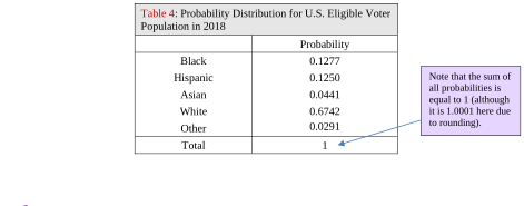
Table 4: Probability Distribution for U.S. Eligible Voter Population in 2018
	Probability
Black	0.1277
Hispanic	0.1250
Asian	0.0441
White	0.6742
Other	0.0291
Total	1

Solution:a)First, we must find the relative frequency for each class.

$$\begin{array}{cc}P\left(\text{GPA }1.5\text{ to }1.99\right)& =\frac{3}{228}\approx 0.0132\\ P\left(\text{GPA }2.0\text{ to }2.49\right)& =\frac{20}{228}\approx 0.0877\\ P\left(\text{GPA }2.5\text{ to }2.99\right)& =\frac{58}{228}\approx 0.2544\\ P\left(\text{GPA }3.0\text{ to }3.49\right)& =\frac{82}{228}\approx 0.3596\\ P\left(\text{GPA }3.5\text{ to }3.99\right)& =\frac{55}{228}\approx 0.2412\\ P\left(\text{GPA }4.0\text{ to }4.49\right)& =\frac{10}{228}\approx 0.0439\end{array}$$

Putting these into Table 6 we have a probability distribution for college grade point averages.

b)Below 2.0 means the GPA is in the 1.5 to 1.99 category. So,

$$\begin{array}{cc}P\left(\text{GPA below }2.0\right)& =\frac{3}{228}\approx 0.0132\end{array}$$

We can say that the probability that one college graduate had a GPA below 2.0 is 0.0132. Or, we can say that about 1.32% of all college graduates have a GPA below 2.0.

c)The group of students graduating with a GPA of at least 3.5 includes all students with a 3.5 to 3.99 GPA and students with a 4.0 to 4.49 GPA. So, we must combine the two groups to get

$$\begin{array}{cc}P\left(\text{Cum laude}\right)& =\frac{55+10}{228}=\frac{65}{228}\approx 0.2851\end{array}$$

Note that we could also have simply added the probabilities for the two classes from the distribution together.

$$\begin{array}{cc}P\left(\text{GPA }3.5\text{ to }3.99\right)+P\left(4.0\text{ to }4.49\right)& \approx 0.2412+0.0439=0.2851\end{array}$$

(We will look at this sort of feature of probability more in section 5.2.)

We can say that the probability that a college student graduated with the cum laude honor is 0.2851. Or, we can say that about 28.51% of all college graduates receive this honor.

d)The probability that a college graduate graduated with a grade point average less than 2.0 was only 0.0132. That is less than 0.05 and is therefore a rare or unusual event.

Graduating cum laude had a probability that was 0.2851, which is larger than 0.05, and so graduating with this honor is not rare or unusual.

Solution:a)0.75 is a number between 0 and 1, so it is a possible probability.

b)1.32 is not between 0 and 1, so it is not a possible probability.

c)-0.17 is not between 0 and 1, so it is not a possible probability.

d)$\frac{12}{55}\approx 0.2812$. So, it is a number between 0 and 1 and could be a probability.

e)$\frac{35}{27}\approx 1.296$, which is not between 0 and 1, so it is not a probability. In fact, any fraction where the numerator is larger than the denominator cannot be a probability!

f)The number $7.23\times {10}^{-3}$ is written in scientific notation. Multiplying a number by ${10}^{-3}$ is the same as dividing it by ${10}^3$. Each time you divide by 10, the number will get smaller as the decimal moves one place to the left. That means that multiplication by ${10}^{-3}$ will move the decimal three places to the left of the original decimal place.

$$\begin{array}{cc}& 7.23\times {10}^{-3}=\frac{7.23}{{10}^3}=\frac{7.23}{1000}=0.00723\mathrm{.}\end{array}$$

Since the decimal is between 0 and 1, it could be a probability.

Solution:Miranda, asks Jasmine “How can I find the probability? It is completely covered in mustard!”

Jasmine calmly replies, “Tell me, what do all the probabilities have to add up to?”

Miranda responds through teary eyes “They are supposed to add up to 1, right?”

“Yes,” Jasmine replies. “And how much do the visible probabilities add up to?”

“Well, the ones that aren’t covered in mustard add up to... let’s see... 0.65.”

0.06 + 0.29 + 0.06 + 0.09 +0.15 = 0.65

“Great!” says Jasmine. “So, now you know the probability that someone prefers TikTok because it’s the only one missing and all the probabilities have to add up to 1.”

“Hey! You are brilliant! The probability that someone prefers TikTok is one minus all the rest!”

Miranda then writes out, $P\left(\mathrm{TikTok}\right)=1-0.65=0.35$.

“Thanks Jasmine! You are the best!”